Wax deposition on pipeline walls is a recurring problem in flow assurance, especially in deep waters.  Fluids containing long aliphatic hydrocarbon chains (C18+) will precipitate as paraffin waxes at temperatures below the Wax Appearing Temperature (WAT), also defined as Cloud Point [1]. Such temperatures can be easily reached in pipes surrounded by low temperature environments, and these conditions can lead to wax deposition on the pipe walls. As a consequence, the deposited layer can increase the required lifting power, restrict the flow and, consequently, result in loss of production or even completely block the pipeline, demanding constant cleaning procedures or eventual replacement of pipe sections.

Besides the operational issues due to wax deposition at the inner walls of the pipe, the cost of applying remedial procedures increases steeply with water depth,making this a crucial problem to solve in order to secure the economic viability in offshore petroleum production [2]. Therefore, accurate models are necessary to estimate deposition so that it can be prevented or reduced  by designing pipelines better. 

In the Oil and Gas industry, simulations are widely used to assist decision making in the design and operations of hydrocarbon fields. The ability to couple complex models with a multiphase flow simulator through a flexible and comprehensive plugin structure API is important in order to create state-of-the-art models and apply them to solve industry problems. Through ALFAsim’s plugin structure and the ALFAsim-SDK [3], it was possible to implement and validate the Matzain model to estimate the thickness of the deposited wax layer.

Simulating Wax Deposition in ALFAsim

Wax Model:

In the literature, there are several models available to predict wax deposition. Most of these models assume that molecular diffusion is the primary mechanism of this phenomenon. The Matzain model [4] was initially considered in ALFAsim because, besides the molecular diffusion, the model also includes the mechanism of shear dispersion, which is a deposit removal mechanism of the particles away from the wall [5].

In the Matzain model, the rate of wax build-up is calculated through an empirical modification of Fick’s law described below:

where:

• δ is the wax deposition thickness at the pipe wall;

• F_w is the wax mass fraction;

• π₁/1+ π₂ represents the shear dispersion and is a function of the porosity of the wax deposit layer, and the Reynolds number (flow regime dependent)

• D_wo is the diffusion coefficient of wax (evaluated with the Wilke-Chang correlation [6])

When the fluid temperature falls below the WAT at the corresponding pressure in the section, the wax particles begin to precipitate and deposit, forming an internal deposited layer on the inside of the pipeline walls. This deposited layer affects the flow in several ways. The first consequence is pipe diameter reduction, which also impacts the effective geometric properties. That is, the area and volume and all the calculations of the multiphase flow associated with it, such as pressure drops, flow regimes, inflow performance behaviour, and others. Second, this internal deposited layer strongly influences the mass balance of the system, since the wax particles precipitate from the bulk oil. Finally, the thermal conductivity and the thickness of the deposited layer change with time, which will affect the heat transfer between the fluids and the outer environment.

Plugin & API

In a nutshell, the customization framework developed in ALFAsim allows the developer to configure internal settings from ALFAsim through the Solver Configuration Hooks and the Solver Hooks, which are pre-defined functions that modify/extend the models and the thermo-hydrodynamic solver.

Particularly with the wax deposition plugin, it is necessary to configure the following settings:

1. Add a new wax phase and field to the ALFAsim multi-field model [7]. 
2. Create variables to store the relevant model information. It is also important to expose some variables as outputs since they are direct results from the plugin. Examples of these plugin internal variables are the wax thickness and the mass fraction of the oil in the deposited layer. 
3. Configure hooks that allow the plugin to change the conservation equations. These hooks are the most important ones, as they will add source terms to the residual function of mass, momentum, and energy conservation equations.
4. Since the wax plugin needs to get user input data, additional application hooks are available to configure the plugin user interface. In this case, only a wax table (.WAX) is required, and it is generated by traditional thermodynamics modelling tools. This table contains information on the wax phase properties and their concentrations at each point of pressure and temperature.

The customization toolkit, named ALFAsim-SDK, assists anyone with programming skills and knowledge in multiphase flow to implement a plugin containing custom (in-house) models of ALFAsim’s framework. It provides a set of tools which allow a developer to create, compile, and bundle a plugin. The available toolkit allows the execution of the following steps:

1. Template: Generates a template with the necessary files and structure to implement a plugin.
2. Compile: Compiles the plugin and creates the artifacts folder containing the compiled files.
3. Package: Generates the plugin itself with the compiled files necessary to install it.

Simulation

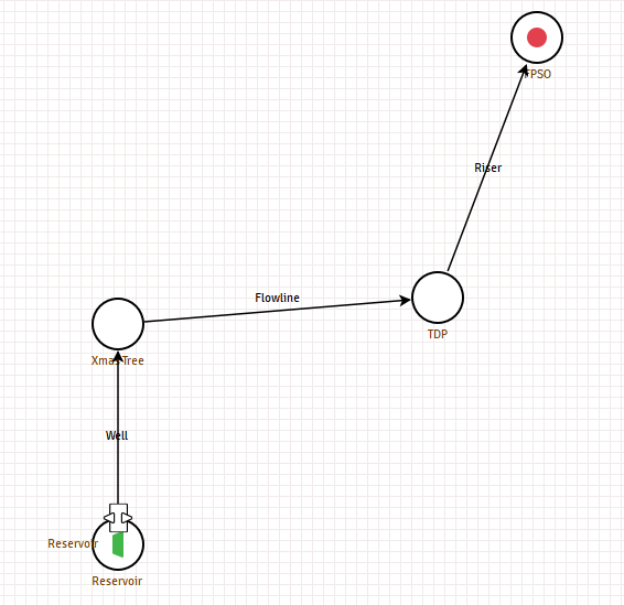
The case simulated represents a simplified production well from a Brazilian pre-salt field. The system consists of a well with approximate length of 4 km and inner diameter (ID) of 5.79 in; a 6-in ID flowline; and a 6-in ID riser (Figure 1). The reservoir boundary conditions include a pressure of 610 bar and a temperature of 69º C with a reservoir inflow producing oil with PI equals 10.5 [sm3/bar.d]. The Christmas tree and TDP (Touch Down Point) temperatures are 40º C and 5º C, respectively. Finally, the surface boundary conditions are a pressure of 20 bar and a temperature of 30º C.

The Figure 2 shows the outer environment temperature profile for the entire pipeline system, and the trajectories of the coupled pipelines, respectively.

A PVT (Pressure-Volume-Temperature) look-up table was built using a commercial thermodynamics modeling simulator in order to represent the fluid properties and phase behavior in the simulation. Similarly, a wax table was built with the same commercial software to represent the wax phase properties and the cloud points. 

Results and Discussions

The deposit thickness is the main result to analyse from the wax plugin. The wax thickness profiles obtained through all trajectories for 3, 12, 35, and 76 days are shown in Figure 4. Upon examination of the curves in the figure, it is possible to infer that the deposition shape remains the same throughout the simulation history. Additionally, the thickness of the deposited layer at the inner wall of the pipeline reaches 2 mm in 76 days. 

Figure 4 shows a plot of the outer environment temperature and the wax thickness at one simulation day. With these data, we can infer that the wax thickness starts to rise exactly when the temperature falls below the cloud point, as shown in the black point in the graphic.

With those simulation results, the flow assurance engineer can decide how to solve the deposition problem. Once it’s known that wax deposition will occur, it’s possible to propose a proper pipeline design with proper insulation at the design stage, while at the production stage, mitigation methods such as pigging, heating,  wax dispersant, pour point depressant, and wax crystal modifiers can be used to keep production economically viable and to avoid major issues such as pipeline blockages. 

Stay tuned for the next blog posts exploring how our simulation tools can help enhance production.

References

[1] Cem Sarica and Michael Volk. Tulsa university paraffin deposition projects. Technical report, The University of Tulsa (US), 2004.

[2] LFA Azevedo and AM Teixeira. A critical review of the modeling of wax deposition mechanisms. Petroleum Science and Technology, 21(3-4):393–408, 2003.

[3] ESSS (2020). ALFAsim-SDK Documentation. Available at <https: //alfasim-sdk.readthedocs.io>. Accessed in February 2020.

[4] Matzain, A., Zhang, H. Q., Volk, M., Redus, C. L., Brill, J. P., Apte, M. S., & Creek, J. L. (2000, July). Multiphase flow wax deposition modeling. In BHR Group Conference Series Publication (Vol. 40, pp. 415-444). Bury St. Edmunds; Professional Engineering Publishing; 1998.

[5] Giacchetta, G., Marchetti, B., Leporini, M., Terenzi, A., Dall’Acqua, D., Capece, L., & Grifoni, R. C. (2019). Pipeline wax deposition modeling: A sensitivity study on two commercial software. Petroleum, 5(2), 206-213.

[6] Wilke, C. R., & Chang, P. (1955). Correlation of diffusion coefficients in dilute solutions. AIChE Journal, 1(2), 264-270.

[7] Bonizzi, M., Andreussi, P., & Banerjee, S. (2009). Flow regime independent, high-resolution multi-field modeling of near-horizontal gas-liquid flows in pipelines. International Journal of Multiphase Flow, 35(1), 34-46.